Seamless Stitching of Perfect Labels
The previous articles describe how to unwrap labels programmatically and how we trained a neural network to detect keypoints. This article is about how to stitch multiple images into a single long one.
![]()
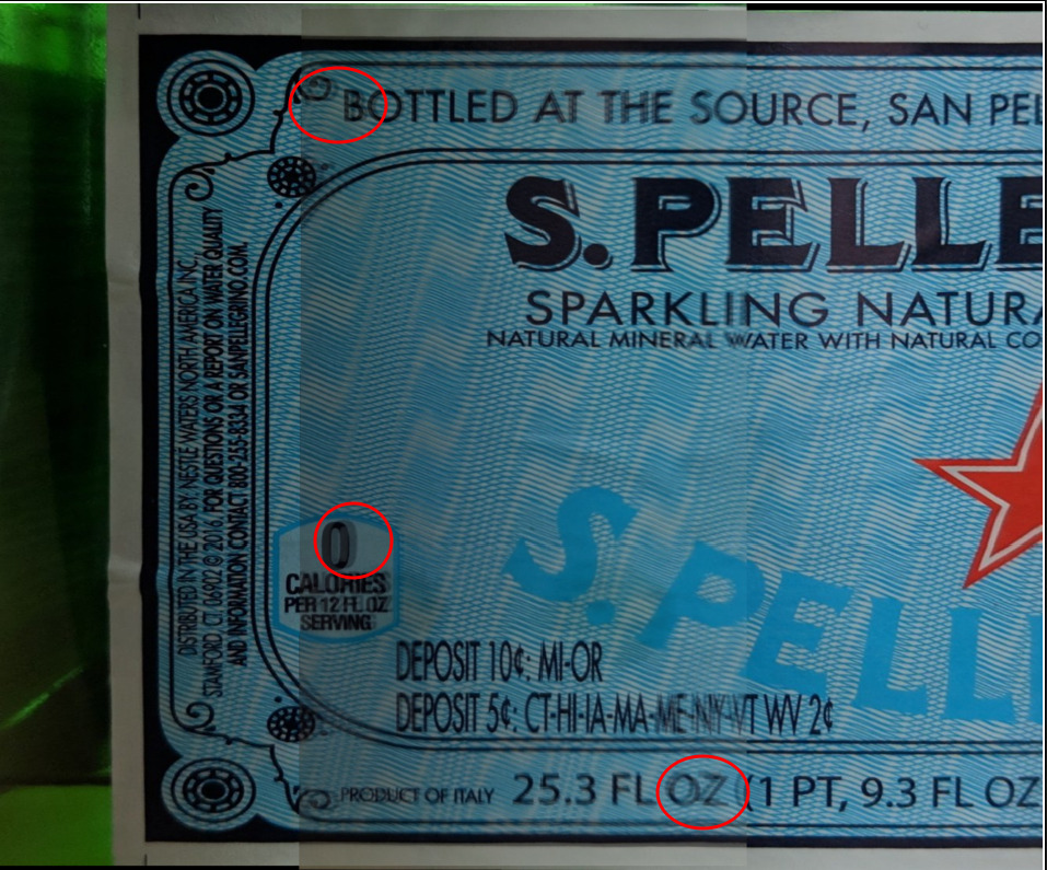
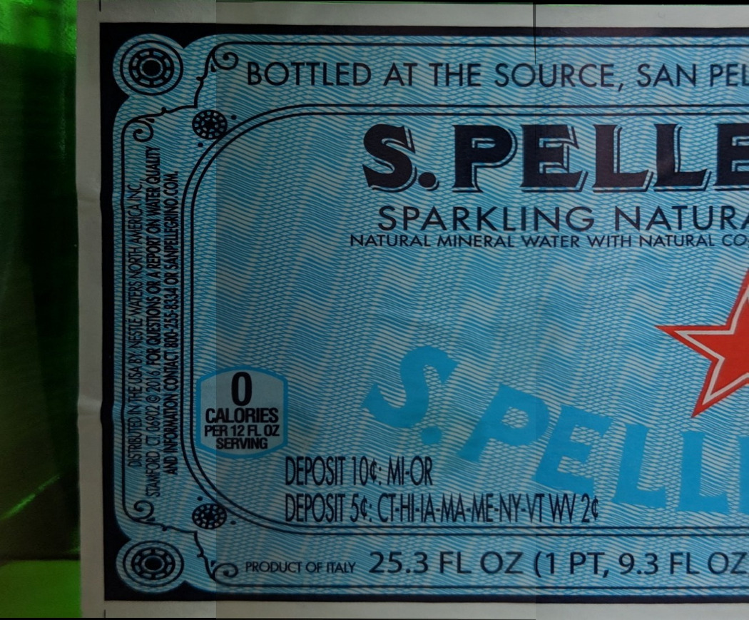
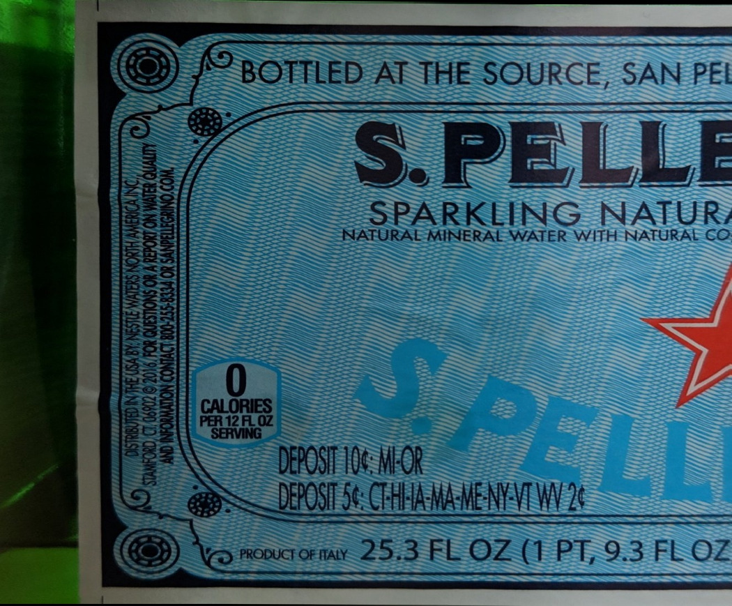
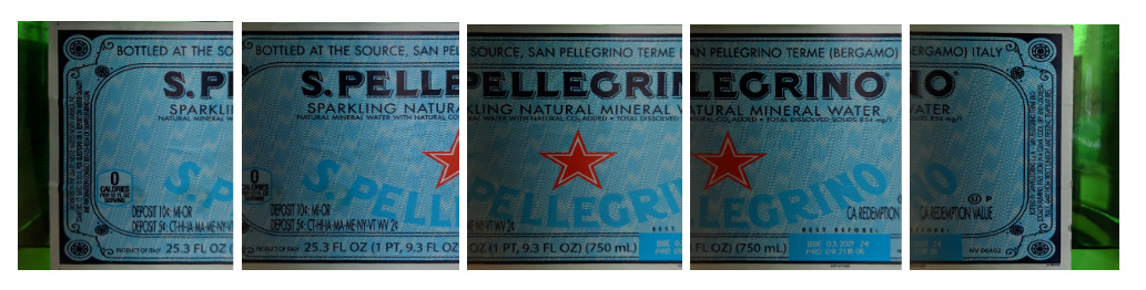
The original set of images (below) was segmented and unwrapped in advance by a neural network, as described in the previous articles. Please see them for more detail.
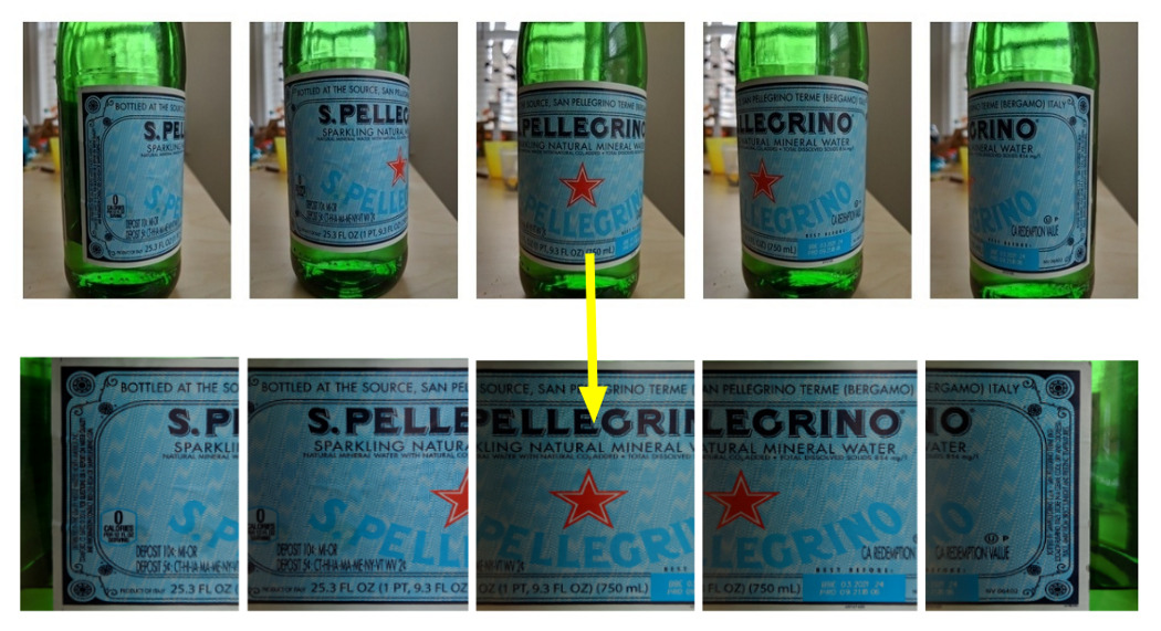
How does stitching even work? We take two images with overlapping areas, compute the mutual shift from each other, and blend them. Sounds pretty easy, but let’s go through each of the steps. To calculate the shift, it’s required to find something that exists on both images, and find a formula to convert points from the first image into points on the second one. The mentioned shift can be represented by a homography matrix, where the cell values encode the different types of transformations together — scaling, translation, and rotation. As we can see, in these photos, there are plenty of common objects:
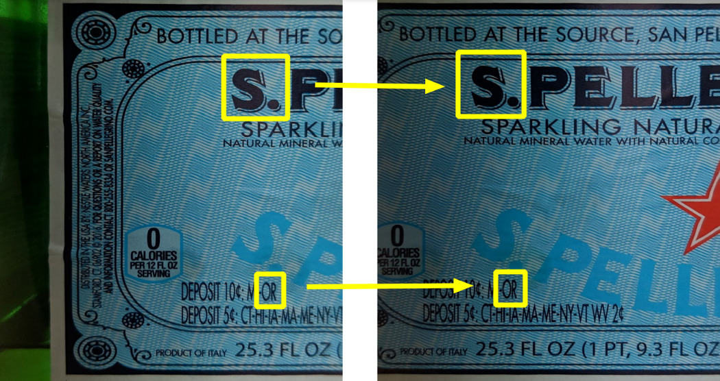
The problem with the given features is that it’s hard to detect them programmatically. Luckily, there are algorithms that detect “good” features (also known as “corners” — there is an excellent document that explains them). One such algorithm is SIFT (Scale-Invariant Feature Transform). Despite being invented in 1999, it’s still very popular due to its simplicity and reliability. Since SIFT is patented, it’s a part of OpenCV non-free build, but the patent recently expired (in March 2020), so it will probably become a part of standard OpenCV soon. Now, let’s find similar features on both images:
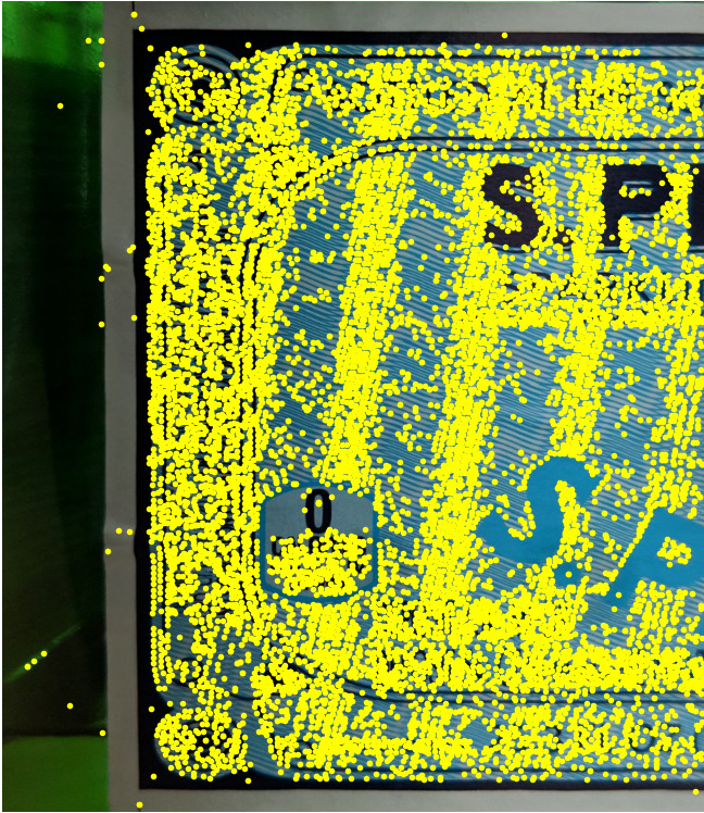
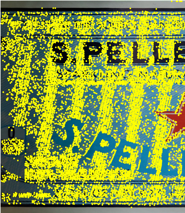
Using a Flann based matcher can find matches relatively quickly between two images, despite a large number of corners. The yellow lines in the picture below connect similar features in the left and right images.
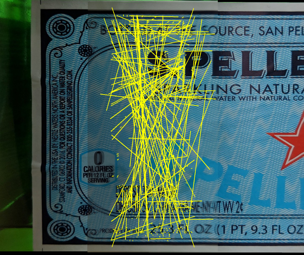
For clarity, the images were placed above each other with the proper offset (which is calculated at a later point in the process, rather than here). As it’s easy to see, there are still lots of mismatches — about 50% of them were wrong. However, the good matches will always generate the same translation, meantime the bad ones will give chaotically different directions. A picture below depicts only the good matches:
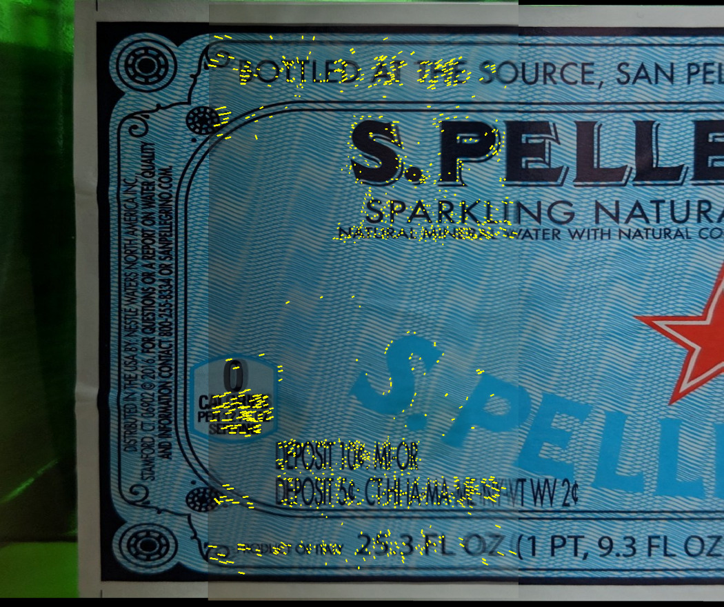
One of the approaches to find a proper translation is a RANSAC algorithm. It goes through the matches iteratively and uses a voting approach to figure out if the proper translation is already found. Luckily, OpenCV provides multiple choices to find homography using RANSAC — the difference between methods is in dimensions of freedom the transformation is going to have. In our case, we need to use estimateAffinePartial2D which will look for the following transformations: rotation + scaling + translation (4 dimensions of freedom).
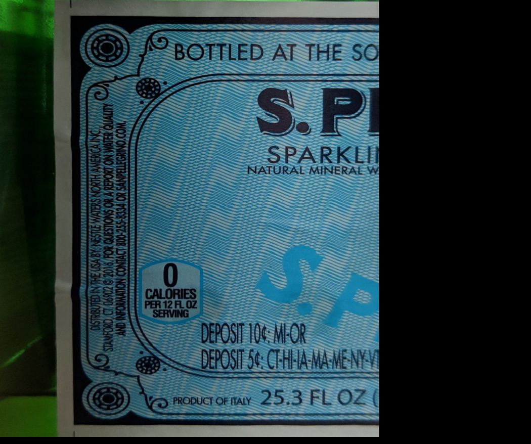
The left image:
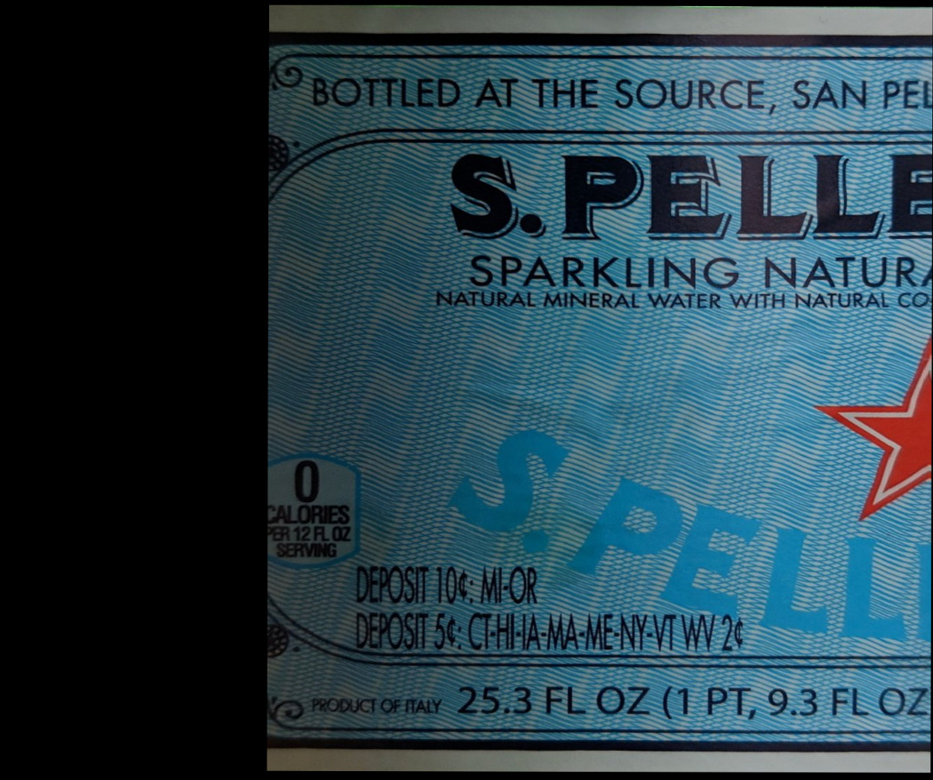
The right image:
Let’s blend them using a naive method, where the intersected region is
calculated as a mean of left and right images. Unfortunately, the result isn’t
really impressive — there are double vision artifacts across the image,
especially closer to stitches.
The animation shows the shift between the tiles:
It’s not surprising — the images were taken from slightly different angles,
and there are tiny differences between them.
For seamless stitching, it’s required to compensate for those non-linear
distortions. The distortion can be described as a smooth vector field, with
the same resolution as the original tiles. This vector field is called
“optical flow”.
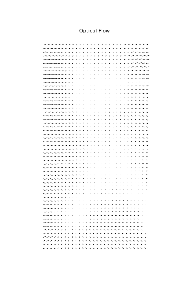
There are several techniques to calculate the flow — with functions that come
with OpenCV or special neural network architectures.
Our optical flow for the given two tiles:
To avoid artifacts during stitching, it’s required to compensate both images
proportionally. For that purpose, we split the optical flow into two matrices:
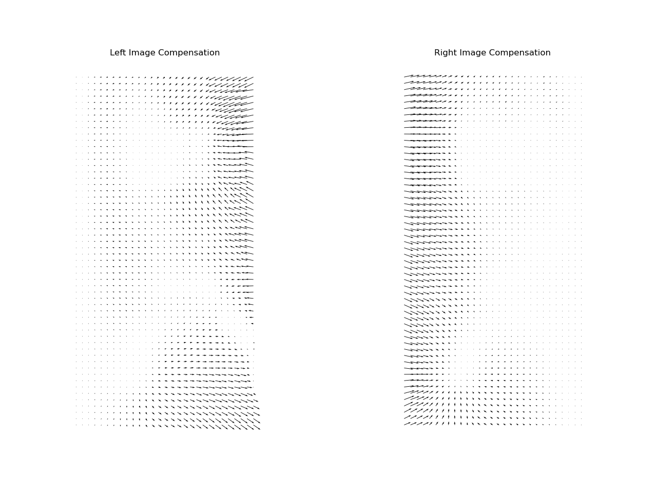
Now the two images are almost perfectly aligned:
Once we blend the full image, it appears to be geometrically correct, but we
observe a brightness jump:
The issue is quite easy to fix if, instead of mean values, we use a blending
formula, where the values are applied with the gradient:
With that approach, the stitching is absolutely seamless:
There are other blending algorithms that work well with panorama stitching (such as multiband blending), but they don’t work well for images with text — only optical flow compensation can completely remove ghosting on characters.
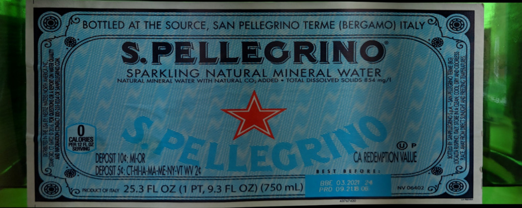
Let’s stitch the entire set of images:
The final result:
Future improvements could be a shadow effect compensation (the right side of the image), and even doing more post-processing to improve colors and contrast. Here we learned how stitching works, and how to make it seamless for production use. The service is available for everyone at Perfect Label as a REST API.
The recommended links:
- SIFT explained https://docs.opencv.org/master/da/df5/tutorial_py_sift_intro.html
- OpenCV homography explained https://docs.opencv.org/master/d9/dab/tutorial_homography.html
- Panorama Autostitching http://matthewalunbrown.com/papers/ijcv2007.pdf
- OpenPano https://github.com/ppwwyyxx/OpenPano
- Google Photo Scanner https://ai.googleblog.com/2017/04/photoscan-taking-glare-free-pictures-of.html